



Education Content Expert
Least Square Method is a process of finding the best-fitted line for any data set that is described by an equation. Least Square Method requires reducing the sum of squares of the residual parts of the points from the curve or line and the trend of outcomes is found quantitatively. This process is also called regression analysis.
Least Square Method is the method of fitting equations that derives the curves to given raw data. The fitting of curves for a particular data set is not always unique. Thus, we need to find a curve having a minimal deviation from all the measured data points. This is called the best-fitting curve and is found by using the least square method.
| Table of Content |
Key Terms: Least Square Method, Regression, Equation, Independent Variables, Ordinary Least Square, Deviation, Least Square Method Formula
Least Square Method Definition
[Click Here for Sample Questions]
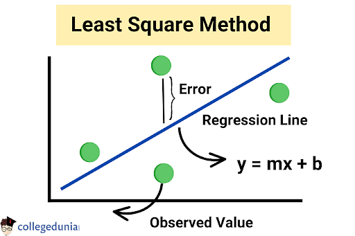
Least Square Method is a statistical method that is used to find a regression line or a best-fit line for the given pattern. Least Square Method defines the solution for the minimization of the sum of squares of deviations or the errors in the result of each equation. The best fit result is assumed to lower the errors and the sum of their squares. The sum of the squares of the errors helps in finding the variation of the equation.
For example, we have 4 data points, and using the least square method we arrive at the following graph:
Least Square Method
Read More:
| Relevant Concepts | ||
|---|---|---|
| Multiple Regression | Linear Regression | Probability and Statistics Symbols |
| Bivariate Analysis | Coefficient of Determination Formula | Linear Regression Formula |
Least Square Method Formula
[Click Here for Sample Questions]
Least Square Method refers to the curve that best fits a set of observations with a minimum sum of errors. Let us assume that the given data points are (x1, y1), (x2, y2), (x3, y3), …, (xn, yn) in which all x’s are independent variables, and y’s are dependent ones.
Least Square Method is used to find a linear line of the form y = mx + b, where y and x are variables, m is the slope, and b is the y intercept. The formula to calculate slope m and the value of b is given by:
m = (n∑xy - ∑y∑x)/n∑x2 - (∑x)2
b = (∑y - m∑x)/n
Here, n refers to the number of data points.
The steps to calculate the least square using the Least Square Method formula are:
- Step 1: Create a table with 4 columns where the first two columns are for x and y points.
- Step 2: Find xy and (x)2 in the next two columns.
- Step 3: Calculate ∑x, ∑y, ∑xy, and ∑(x)2.
- Step 4: Now, find the value of slope m using the above formula.
- Step 5: Next, calculate the value of b.
- Step 6: Lastly, substitute the value of m and b in the equation y = mx + b.
Solved ExampleExample: Consider that we are given the data points as follows:
Ans. In order to find the regression line, we will follow the given steps:
Now, we will find the value of m by using the Least Square Method formula, m = (n∑xy - ∑y∑x)/n∑x2 - (∑x)2 m = [(5×88) - (15×25)]/(5×55) - (15)2 m = (440 - 375)/(275 - 225) m = 65/50 = 13/10 Finding the value of b by using the formula, b = (∑y - m∑x)/n b = (25 - 1.3×15)/5 b = (25 - 19.5)/5 b = 5.5/5 Thus, the required equation of least squares is y = mx + b = 13/10x + 5.5/5. |
Read More: Statistics Important Questions
Least Square Method Graph
[Click Here for Sample Questions]
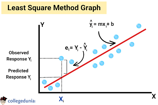
In the graph given below, the straight line shows the potential relationship between the independent variable and the dependent variable. The main goal of the least square method is to reduce this difference between the observed response and the response predicted by the regression line.
There are both vertical residuals and perpendicular residuals. Vertical residual is mostly used in polynomials and hyperplane problems whereas perpendicular is used in general as in the graph given below.
Least Square Method Graph
Types of Least Square Method
[Click Here for Sample Questions]
Least square methods can be classified broadly under 2 categories, depending upon the linearity of the residuals in the equation:
- Linear or Ordinary Least Square: Observed mostly in the regression analysis of statistics.
- Non-linear Least Square: Uses an iterative method to solve the equation, where the equations are assumed to be linear with every iteration.
Uses of Least Square Method
[Click Here for Sample Questions]
Least square method is considered for application in the analysis of the returns of a stock of a company. The analysis is done based on the risks and the returns the stock has are provided in the index. Analysts, then, plot points of returns on a chart and then designate the dependent and independent variables and the best fit line on this chart helps to make calls on buying or selling the stock.
Apart from this, the least square method is also used in various real-life activities such as
- In medicines to mark the side effects of a particular drug.
- Study of the correlation between investment and sales as considered from the economics point of view.
- Study of the measured data.
Also Check:
| Related Topics | ||
|---|---|---|
| Correlation Coefficient Formula | Differences between Correlation and Regression | R Squared |
| Data Sets | Average Deviation Formula | Mean of Grouped Data |
Limitations of the Least Square Method
[Click Here for Sample Questions]
Least square method is the best fit curve to decide the results, however, it has some drawbacks which have been listed below:
- Least square method assumes the errors in the independent variables to be zero, however, this should not be the case as these errors are not zero in real life.
- Least square method is applicable for two variables only.
- It is unreliable when the data is scattered unevenly.
Read More: Statistics Revision Notes
Things to Remember
- Least Square Method is a statistical method used to find the line of best fit of the form of an equation to the given data.
- The best fit line can be any curve that minimizes the error of the given equation.
- Least Square Method is used to predict the behavior of the dependent variable in relation to the independent variable.
- There are two types of least square methods namely linear and nonlinear least squares.
- The main aim of the Least Square Method is to minimize the sum of the squared errors.
- Least square method is often applied in data fitting.
Sample Questions
Ques. Consider the given set of points: (1, 1), (-2,-1), and (3, 2). Use the least square method in order to determine the equation of a line of best fit for the data. (5 Marks)
Ans. There are three points given to us, so the value of n is 3.
| x | y | xy | x2 |
|---|---|---|---|
| 1 | 1 | 1 | 1 |
| -2 | -1 | 2 | 4 |
| 3 | 2 | 6 | 9 |
| ∑x = 2 | ∑y = 2 | ∑xy = 9 | ∑x2 = 14 |
Find the value of m, using the least square method formula.
m = (n∑xy - ∑y∑x)/n∑x2 - (∑x)2
m = [(3×9) - (2×2)]/(3×14) - (2)2
m = (27 - 4)/(42 - 4)
m = 23/38
Find the value of b using the formula,
b = (∑y - m∑x)/n
b = [2 - (23/38)×2]/3
b = [2 -(23/19)]/3
b = 15/(3×19)
b = 5/19
Thus, the required equation of least squares is calculated as y = mx + b = 23/38x + 5/19.
Ques. Are Least Squares the same as Linear Regression? (2 Marks)
Ans. No, linear regression and least squares are not the same concepts. Linear regression refers to the analysis of data in statistics to predict the value of the quantitative variable. On the other hand, least squares is one of the methods that is used in linear regression to find the predictive model.
Ques. Consider the time series data given below:

Use the least square method to determine the equation of a line of best fit for the data. (5 Marks)
Ans. According to the question,
- Mean of xi values = (8 + 3 + 2 + 10 + 11 + 3 + 6 + 5 + 6 + 8)/10 = 62/10 = 6.2
- Mean of yi values = (4 + 12 + 1 + 12 + 9 + 4 + 9 + 6 + 1 + 14)/10 = 72/10 = 7.2
- Straight line equation is y = a + bx.
The normal equations are
∑y = an + b∑x
∑xy = a∑x + b∑x2
| x | y | x2 | xy |
|---|---|---|---|
| 8 | 4 | 64 | 32 |
| 3 | 12 | 9 | 36 |
| 2 | 1 | 4 | 2 |
| 10 | 12 | 100 | 120 |
| 11 | 9 | 121 | 99 |
| 3 | 4 | 9 | 12 |
| 6 | 9 | 36 | 54 |
| 5 | 6 | 25 | 30 |
| 6 | 1 | 36 | 6 |
| 8 | 14 | 64 | 112 |
| ∑x = 62 | ∑y = 72 | ∑x2 = 468 | ∑xy = 503 |
Substituting these values in the normal equations,
10a + 62b = 72….(1)
62a + 468b = 503….(2)
(1) × 62 – (2) × 10,
620a + 3844b – (620a + 4680b) = 4464 – 5030
-836b = -566
b = 566/836
b = 283/418
b = 0.677
Substituting b = 0.677 in equation (1),
10a + 62(0.677) = 72
10a + 41.974 = 72
10a = 72 – 41.974
10a = 30.026
a = 30.026/10
a = 3.0026
Therefore, the equation becomes,
y = a + bx
y = 3.0026 + 0.677x.
Ques. Given data shows the sales (in million dollars) of a company.

Estimate the sales in the year 2020 using the regression line. (5 Marks)
Ans. Here, there are 5 data points. So n = 5.
Here, we will use the substitution t = x-2015 to make the given data manageable. Here, t represents the number of years after 2015.
| x | y | xy | x2 |
|---|---|---|---|
| 0 | 12 | 0 | 0 |
| 1 | 19 | 19 | 1 |
| 2 | 29 | 58 | 4 |
| 3 | 37 | 111 | 9 |
| 4 | 45 | 180 | 16 |
| ∑x =10 | ∑y = 142 | ∑xy = 368 | ∑x2 = 30 |
Finding the value of m using the formula,
m = (n∑xy - ∑y∑x)/n∑x2 - (∑x)2
m = [(5×368) - (142×10)]/(5×30) - (10)2
m = (1840 - 1420)/150 - 100
m = 42/5
m = 8.4
Now, calculating the value of b using the formula,
b = (∑y - m∑x)/n
b = (142 - 8.4×10)/5
b = (142 - 84)/5
b = 11.6
Thus, the equation of least squares is y(t) = 8.4t + 11.6.
Now, for 2020, the value of t will be 2020 - 2015 = 5
The estimation of the sales in the year 2020 is given by substituting 5 for t in the calculated equation,
y(t) = 8.4t + 11.6
y(5) = 8.4×5 + 11.6
y(5) = 42 + 11.6
y(5) = 53.6
Thus, the predicted number of sales in 2020 is $53.6 million.
Ques. Fit a least square line for the given data. Also, find the trend values and show that
∑(Y–Yˆ)=0
∑(Y–Y^)=0. (3 Marks)

Ans.
| X | Y | XY | X2 | Y^=1.1+1.3X | Y–Y^ |
|---|---|---|---|---|---|
| 1 | 2 | 2 | 1 | 2.4 | -0.4 |
| 2 | 5 | 10 | 4 | 3.7 | +1.3 |
| 3 | 3 | 9 | 9 | 5.0 | -2 |
| 4 | 8 | 32 | 16 | 6.3 | 1.7 |
| 5 | 7 | 35 | 25 | 7.6 | -0.6 |
| ∑X=15 | ∑Y=25 | ∑XY=88 | ∑X2=55 | Trend Values | ∑(Y–Y^)=0 |
The equation of least square line:
Y=a+bX
Y=a+bX
Normal equation for ‘a’ ∑Y = na+b∑X 25 = 5a+15b — (1)
Normal equation for ‘b’ ∑XY = a∑X+b∑X2 88 = 15a+55b —(2)
Eliminate a from eq (1) and (2), then multiply equation (2) by 3 and subtract from equation (2). Hence, we get the values of a and b.
Here a=1.1 and b=1.3, so the equation of the least square line becomes
Y=1.1+1.3X
Ques. Fit the straight line to the following data. (3 Marks)

Ans. Σy = aΣx + nb and
Σxy = aΣx2 + bΣx
Now,
| x | y | x2 | xy |
|---|---|---|---|
| 1 | 1 | 1 | 1 |
| 2 | 2 | 4 | 4 |
| 3 | 3 | 9 | 9 |
| 4 | 4 | 16 | 16 |
| 5 | 5 | 25 | 25 |
| Σx = 15 | Σy = 15 | Σx2 = 55 | Σxy = 55 |
Substituting in the equations,
15 = 15a + 4b and 55 = 55a + 15b
Solving these two equations, we get a=1 and b=0,
Hence, the desired curve of best fit is y=x
Ques. If the equation y=axb can be written in linear form Y=A+BX, what will be Y, X, A, B? (3 Marks)
Ans. The curve given is y=axb.
Taking log on both sides, we have,
Log y = log a + b log x.
It can be written as Y=A+BX,
Where
Y=log y, A=log a, B=b, and X=log x
Ques. Fit the straight-line curve to the following data. (3 Marks)

Ans. The normal equation are:
Σy = aΣx + nb
and
Σxy = aΣx2 + bΣx.
Substituting the values, we get,
819 = 798a + 10b
66045 = 64422a + 798b
Solving, we get
a = 0.9288 and b = 7.78155
Therefore, the straight line equation is :
y = 0.9288x + 7.78155
Ques. What is Least Square Method Formula? (3 Marks)
Ans. In order to determine the equation of the line for any data, we need to use the equation y = mx + b. The least square method formula is calculated by finding the value of both m and b by using the formulas:
- m = (n∑xy - ∑y∑x)/n∑x2 - (∑x)2
- b = (∑y - m∑x)/n
Here n denotes the number of data points.
Ques. What do you mean by Least Square Method in Regression? (2 Marks)
Ans. The least square regression helps to calculate the best fit line of the set of data from both the activity levels and corresponding total costs. The idea to use the method and calculation is to minimize the sum of the squares of the vertical errors between the data points and cost function.
Ques. What is Least Square Curve Fitting? (1 Mark)
Ans. Least square method refers to the process of fitting a curve according to the given data. The method is used to determine the trend line for the given data.
Check-More:



Comments